AI inventory replenishment uses predictive models to estimate future demand and then combines those forecasts with actual inventory position, supplier lead times, safety stock, ordering constraints and risk controls to recommend when and how much stock to reorder.
The important distinction is that forecasting demand is not the same thing as deciding to buy inventory.
A model might predict that a distributor will sell 300 units of a product over the next two weeks. That does not mean the business should order 300 units. It may already have 180 units on hand, another 100 inbound from a supplier, a minimum order quantity of 50 and enough safety stock to cover normal demand variability.
A safe replenishment system therefore needs a decision chain:
Demand forecast → inventory position → supplier lead time → safety stock → purchasing constraints → reorder recommendation → approval or automationThat is where predictive inventory becomes operationally useful.
It is also where AI inventory reordering becomes more complicated than many descriptions of “AI-powered forecasting” imply.
At AIMEC, we built a small replenishment lab using synthetic-but-realistic catalogue, order and inventory data to test this distinction. We compared a transparent reorder-point baseline with a predictive approach across the same unseen historical periods.
The predictive approach improved aggregate service level from 90.81% to 92.26%, reduced simulated lost demand from 936 to 789 units and lowered forecast error from 36.11 to 29.19 units, while average inventory remained relatively similar at 63.60 units for the baseline and 64.75 for the predictive policy.
However, the predictive approach did not win on every metric. It recorded more stockout days overall and performed materially worse on the cold-start SKU. That mixed result is exactly why replenishment systems should be evaluated at both portfolio and SKU level before purchasing decisions are automated.
What Is Predictive Inventory Replenishment?
Predictive inventory replenishment is a system for estimating future stock requirements and turning those estimates into reorder recommendations.
AI or machine learning usually sits in the forecasting part of the system. It can learn relationships between historical sales, seasonality, changing demand velocity, promotions, customer behaviour and other signals to estimate what demand may look like during the period in which new stock would need to arrive. But the forecast is only one input.
A replenishment engine still has to answer two operational questions:
| Question | Example |
| When should we reorder? | When inventory position falls below expected lead-time demand plus the required safety stock. |
| How much should we order? | Enough to restore an appropriate inventory position while respecting MOQ, supplier and purchasing constraints. |
The distinction matters because even an excellent demand forecast can produce a bad purchasing decision if the system has an incorrect stock count, ignores incoming inventory or uses the wrong supplier lead time.
Forecasting Demand Is Not the Same as Deciding What to Order
Consider a product with predicted demand of 200 units during the next 10 days. A simplistic “AI orders what it predicts” system might recommend buying 200. Now add the operational data.
The warehouse has 120 units physically available. Another 60 units are due from an existing purchase order. Twenty units are already allocated to outstanding customer orders. The supplier only accepts orders in multiples of 50. The business also wants a safety buffer of 40 units.
The purchasing decision is no longer 200 units.
The system first needs to calculate the effective inventory position and then determine whether that position will adequately cover expected demand and the safety-stock requirement until replenishment arrives.
That decision flow should look more like this:
Orders / Sales History

        ↓

Demand Features

        ↓

Demand Forecast

        ↓

Current Available Inventory

        ↓

Allocated / Reserved Stock

        ↓

Inbound Purchase Orders

        ↓

Supplier Lead Time

        ↓

Safety Stock

        ↓

MOQ / Order Multiples / Supplier Rules

        ↓

Proposed Reorder Quantity

        ↓

Risk & Confidence Controls

        ↓

Auto-approve | Human Review | Block

        ↓

ERP / Procurement / Inventory System
The model predicts. The replenishment policy decides.
The Data an AI Inventory Replenishment System Actually Needs
Sales history is the obvious starting point, but production replenishment requires considerably more.
A practical SKU-level record might look like this:
| Field | Purpose |
| sku | Identifies the item being replenished |
| daily_sales | Historical demand signal |
| on_hand_qty | Physical stock available |
| allocated_qty | Stock committed to existing orders |
| available_qty | Inventory currently available for sale |
| inbound_qty | Stock already ordered but not received |
| supplier_lead_days | Time required for replenishment to arrive |
| moq | Minimum supplier order quantity |
| order_multiple | Required purchasing increment |
| unit_cost | Supports purchase-value risk controls |
| promotion_flag | Known future demand driver |
| supplier_id | Connects recommendation to purchasing rules |
| warehouse_id | Identifies the inventory location |
The difficult part is usually not accessing the data. It is deciding which quantities mean what, establishing reliable lead-time data and making sure incoming orders, allocations, returns, bundles and stock transfers are represented consistently.
Bad inventory data passed into a more sophisticated model simply produces a more sophisticated bad decision.
The same principle applies to product intelligence more broadly. Businesses already building an AI product catalogue assistant can reuse structured SKU, product relationship and catalogue data as inputs into replenishment systems.
How Traditional Reorder Points Work
Before adding AI, a business should establish a rule-based baseline.
A common approach is:
Reorder point = expected demand during lead time + safety stock
Suppose a SKU sells an average of 12 units per day and takes seven days to arrive from its supplier.
Expected lead-time demand is:
12 × 7 = 84 units
If the business holds 25 units of safety stock, its reorder point becomes:
84 + 25 = 109 units
When effective inventory position reaches approximately 109 units, the replenishment process is triggered.
Safety stock exists because average demand is not guaranteed demand. Variability in demand and lead time increases the amount of protection a business may need.
The important point for an AI project is that this basic rule is not primitive or obsolete.
For a stable product with consistent demand, reliable stock counts and predictable suppliers, a straightforward reorder point can be remarkably difficult for a predictive model to beat once complexity, maintenance and explainability are taken into account.
That makes it an excellent benchmark. If an AI system cannot outperform a simple policy under the same historical conditions, there is little justification for automating purchasing with it.
Where AI Can Improve the Decision
The case for AI becomes stronger when the assumptions behind a static average start breaking down.
Imagine a wholesaler whose product typically sells 20 units a day but has recently accelerated from 15 to 30. A trailing average can be slow to react. A model that recognises the change in demand velocity may estimate lead-time requirements more accurately.
Seasonality creates a similar problem. Demand may differ substantially by weekday, month or trading season.
Promotions can make historic averages even less representative. If a business already knows that a promotion starts next week, that future event is relevant information that a model can incorporate before the sales spike appears in the historic average.
Other products behave intermittently, with many zero-demand periods followed by large B2B orders. In that environment, conventional regression models can perform badly, and specialised intermittent-demand techniques or simple inventory rules may be more appropriate.
The central question is therefore not:
“Can AI forecast this SKU?”
It is:
“Does the predictive approach produce a better inventory decision than the existing policy for this type of SKU?”
That requires a backtest.
AIMEC Labs: Predictive Reordering With Ecommerce and Wholesale Data
To test the full replenishment decision rather than forecasting accuracy alone, AIMEC ran a reproducible inventory replenishment backtest using synthetic-but-realistic data.
The dataset contained 240 days of demand for six SKU profiles: stable, trending, weekly-seasonal, intermittent, promotion-sensitive and cold-start.
The evaluation period ran from 27 March to 14 August 2026, with 99 days of historical information available before the backtest began.
Both policies were evaluated against exactly the same demand periods.
The predictive policy used Ridge regression with features derived from recent demand, seven- and 28-day averages, demand changes, variability, trends, weekday patterns and known promotion signals. The model was refitted every seven days.
To prevent future leakage, each training example was only admitted after its complete lead-time demand window had already occurred. In other words, the model could only learn from information that would genuinely have been available on the decision date.
This was a lab backtest using synthetic data, not a production deployment or ROI study. Supplier lead times were fixed, and the simulation did not model returns, substitutions, stock transfers, supplier capacity constraints or multi-warehouse routing.
Baseline method
The rule baseline estimated lead-time demand from recent sales history and added a safety-stock allowance based on recent demand variability.
A reorder was triggered when inventory position fell below that level. MOQ constraints were then applied to the proposed purchase quantity.
Predictive method
The predictive version used a small regularised regression model rather than a large black-box model.
Features included recent demand, seven- and 28-day averages, recent demand change, demand variability, trend, day-of-week signals and known upcoming promotion periods.
The point of the experiment was not to find the most sophisticated forecasting algorithm possible.
It was to establish whether a modest predictive layer could add value over a transparent rule.
Purchasing controls
The test did not treat every reorder recommendation as automatically executable.
A recommendation was routed for human approval when its simulated purchase value reached the test’s $10,000 approval threshold, forecast confidence fell below 0.55, the SKU was still in its cold-start period, or recent demand variability exceeded the configured risk threshold.
These thresholds were part of the AIMEC lab configuration rather than universal purchasing rules. In a production implementation, they would need to be set according to the organisation’s purchasing authority, inventory value, supplier risk and tolerance for forecast uncertainty.
Baseline vs Predictive Results
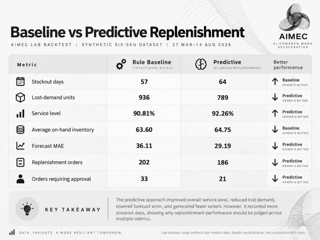
The aggregate backtest produced the following results:
| Metric | Rule baseline | Predictive approach | Result |
| Stockout days | 57 | 64 | Baseline had fewer stockout days |
| Lost-demand units | 936 | 789 | Predictive reduced lost demand by 15.7% |
| Service level | 90.81% | 92.26% | Predictive improved service by 1.45 percentage points |
| Average on-hand inventory | 63.60 | 64.75 | Inventory levels remained broadly similar |
| Forecast MAE | 36.11 | 29.19 | Predictive forecast error was about 19.2% lower |
| Replenishment orders | 202 | 186 | Predictive generated fewer orders |
| Orders requiring approval | 33 | 21 | Predictive produced fewer approval-routed orders |
The overall result favoured the predictive approach on several important measures, but it was not an across-the-board win.
Service level increased from 90.81% to 92.26%, while simulated lost demand fell by approximately 15.7%. Forecast mean absolute error also fell from 36.11 to 29.19 units, an improvement of roughly 19.2%.
Importantly, those improvements did not come from simply carrying dramatically more stock. Average on-hand inventory increased only from 63.60 to 64.75 units, or approximately 1.8%.
The predictive policy also generated 186 replenishment orders compared with 202 for the baseline.
However, stockout days moved in the opposite direction: the predictive policy recorded 64 versus 57 for the baseline.
This apparent contradiction is useful. A stockout day is a binary measure — either a SKU experienced unmet demand that day or it did not. Lost-demand volume measures the size of the shortage. In this simulation, the predictive system experienced shortages on more individual days but reduced the total quantity of demand that could not be fulfilled.
That is why inventory performance should not be judged using a single metric.
Where the predictive model did help
The clearest predictive win came from the promotion-sensitive SKU.
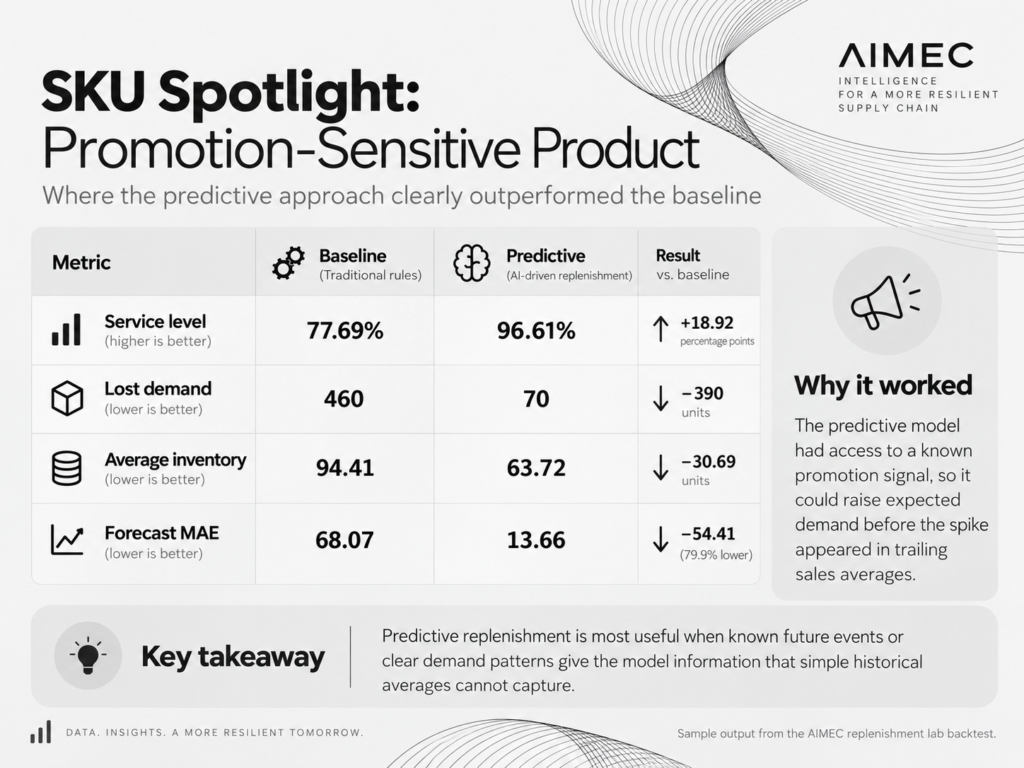
Under the rule baseline, service level was 77.69% and simulated lost demand reached 460 units. The predictive policy increased service level to 96.61% and reduced lost demand to 70 units.
Average inventory also fell from 94.41 units under the baseline to 63.72 under the predictive policy, while forecast MAE fell from 68.07 to 13.66 units.
The reason is important. The predictive model had access to a known upcoming promotion signal. It therefore did not need to wait for the increase in demand to appear in a trailing sales average before responding.
The weekly-seasonal SKU also showed a smaller predictive advantage. Service level increased from 97.94% to 99.24%, while lost demand fell from 38 to 14 units.
These results illustrate where predictive replenishment can be useful: when there is meaningful structure or known information that a simple trailing-demand rule cannot represent well.
Where AI was worse
The cold-start SKU produced the clearest failure in the test.
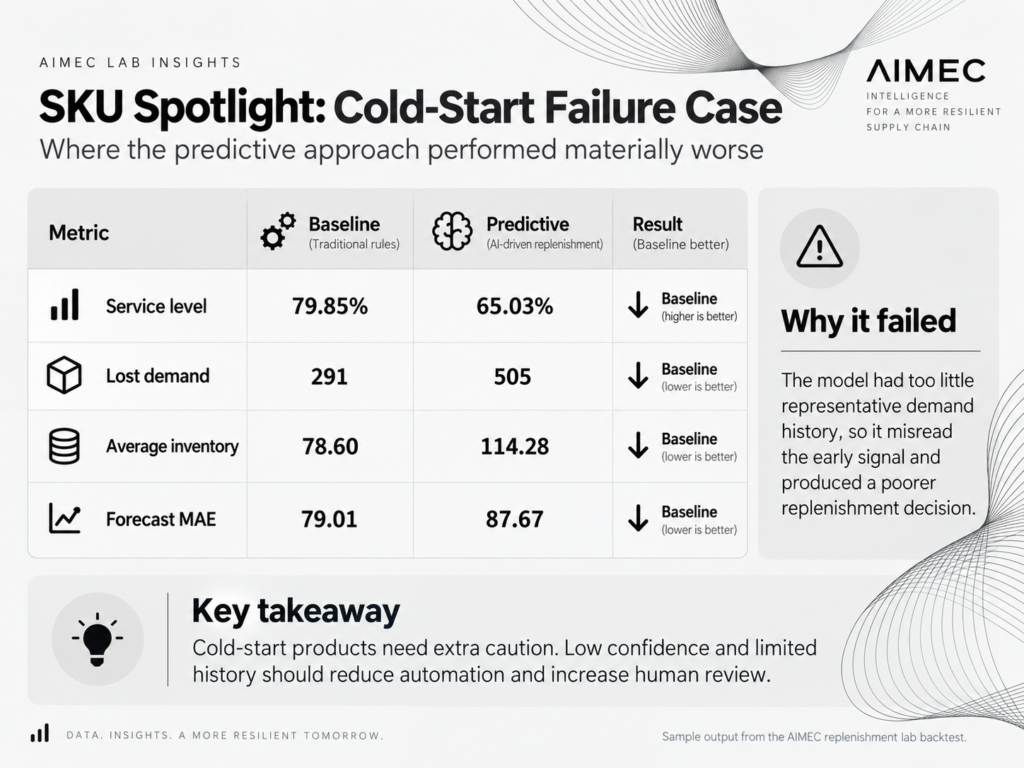
The baseline achieved a 79.85% service level with 291 units of simulated lost demand. The predictive policy fell to a 65.03% service level while lost demand increased to 505 units.
It also carried substantially more inventory. Average on-hand inventory increased from 78.60 units under the baseline to 114.28 under the predictive policy.
Forecast accuracy deteriorated as well, with MAE rising from 79.01 to 87.67 units.
The model had too little representative demand history from which to infer what normal future demand should look like. This is exactly the kind of situation where low confidence should reduce automation rather than increase it.
The intermittent SKU produced a different result. Both policies achieved 100% service with zero lost demand, meaning the predictive model provided no operational service-level advantage. Its forecast MAE was also slightly worse at 22.10 units compared with 21.20 for the baseline.
Stable and trending demand provided additional warnings against assuming predictive automatically means better. The baseline achieved 98.00% service on the stable SKU compared with 96.23% for the predictive policy, while the trending SKU produced 95.62% under the baseline and 94.72% under prediction.
The lesson is not that predictive forecasting cannot handle these demand profiles. It is that this particular predictive method did not improve them. Model choice and SKU segmentation matter.
Should AI Automatically Place the Purchase Order?
Not by default. A useful inventory system can operate at several levels of autonomy.
A low-value SKU with predictable demand, stable lead time, clean inventory data and a model that has demonstrated reliable historical performance may eventually be suitable for automatic approval.
A $5,000 purchase recommendation for a new product with little historical demand is a very different decision. The system should therefore calculate a risk state alongside the reorder quantity.
For example:
{

  "date": "2026-04-23",

  "sku": "SKU-COLD",

  "profile": "cold_start",

  "policy": "predictive",

  "available_qty_before_demand": 28,

  "inbound_qty": 0,

  "supplier_lead_days": 14,

  "forecast_lead_time_demand": 0.0,

  "safety_stock": 56.99,

  "reorder_point": 56.99,

  "inventory_position": 28,

  "recommended_order_qty": 30,

  "moq": 25,

  "unit_cost_usd": 120.0,

  "purchase_value_usd": 3600.0,

  "forecast_confidence": 0.45,

  "decision": "human_approval_required"

}
This example is particularly useful because the purchase value itself was only $3,600 — below the lab’s $10,000 high-value approval threshold.
The recommendation was nevertheless routed to human approval because the predictive system assigned only 0.45 confidence and the SKU was in a cold-start state.
That demonstrates why purchasing controls should consider more than transaction value. Low-confidence predictions, insufficient history and unusual demand conditions can justify review even when the monetary exposure is relatively modest.
This is where human-in-the-loop approval becomes valuable: the system can automate predictable, low-risk decisions while escalating uncertain or financially significant recommendations to a person.
How Predictive Replenishment Fits Into an Ecommerce or Wholesale Architecture
The inventory platform, ERP or ecommerce system should generally remain the system of record for orders, catalogue information and stock. The predictive logic can sit in a separate decision layer.
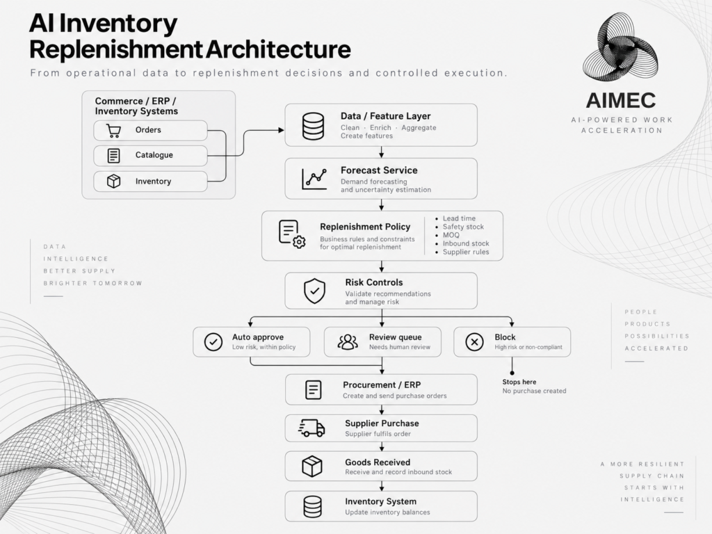
This separation is useful because forecasting, inventory policy and purchasing approval have different responsibilities.
The forecasting service answers: What demand is likely during the replenishment window?
The inventory policy answers: Given our actual inventory position, how much should we order?
The risk layer answers: Should this recommendation be executed automatically?
The procurement system answers: How is the approved order actually placed and tracked?
Keeping those responsibilities separate makes the system easier to test, audit and modify. It also prevents an experimental forecasting model from becoming directly responsible for financial transactions.
For businesses already building product and ordering intelligence, this architecture can share the same foundational data.
A catalogue intelligence system may already understand product relationships, substitutions, categories and customer behaviour.
An order intelligence layer may already understand purchasing patterns, repeat customers and changing demand.
This can also connect with systems designed to automate B2B orders from WhatsApp, where confirmed customer orders become another source of structured demand data for downstream inventory decisions.
Those signals can become features for replenishment without requiring the forecasting model to control the entire commerce stack.
Common Failure Modes in AI Inventory Reordering
The model is often not the first thing that fails.
Incorrect stock counts
If the system believes 500 units exist when the warehouse actually contains 350, even a perfect demand forecast produces the wrong purchasing decision.
Incorrect supplier lead times
A supplier that historically delivered in five days but now takes 14 requires a materially different inventory policy even if customer demand has not changed.
Cold-start products
New SKUs have little historical information. A model can interpret an early surge in demand as a long-term pattern and over-order aggressively.
Promotions
Historic averages may be irrelevant during promotions, launches or unusual campaigns. Known future events should be included where possible rather than expecting the model to infer something that has never happened before.
Returns
Returned products may or may not become sellable inventory again. If the system assumes every return immediately replenishes inventory, its stock position can become inaccurate.
Bundles and kits
Selling one bundle may consume several underlying component SKUs. A replenishment model operating only on the parent product can miss component shortages.
Supplier changes
Changing supplier can alter lead time, MOQ, unit cost, order multiples and reliability simultaneously.
Stock transfers
Inventory moving between warehouses can temporarily appear unavailable even though it has not left the business. These are systems-engineering problems as much as forecasting problems.
These data, integration and operational constraints are also central considerations when planning broader AI implementation in supply chain environments.
When Simple Reorder Rules Are Better Than AI
The AIMEC lab reinforces an important implementation rule: Some inventory should remain boring.
If demand is stable, the SKU catalogue is small, historical data is sparse or buyers need every recommendation to be immediately explainable, a conventional reorder policy can be the better solution.
The stable SKU in the AIMEC test illustrates this point. The rule baseline achieved a 98.00% service level compared with 96.23% for the predictive policy. Forecast MAE was also lower for the baseline at 10.88 units compared with 12.47.
In other words, adding a predictive model did not improve this already understandable demand pattern. The additional modelling complexity would therefore be difficult to justify based on this test alone.
The intermittent SKU went further: the predictive model was actively worse. Businesses should therefore segment inventory before selecting the replenishment method.
A production system does not need one forecasting model for every SKU.
For example:
| SKU pattern | Potential approach |
| Stable, high-volume | Rule-based reorder point |
| Strong seasonal pattern | Predictive forecasting |
| Trending demand | Predictive forecasting |
| Promotion-sensitive | Predictive model with event inputs |
| New product | Manual or conservative policy |
| Highly intermittent | Specialist model or simple rule |
| High-value purchase | Prediction plus mandatory approval |
Selective intelligence is usually safer than universal automation.
A Practical Implementation Roadmap
1. Clean the inventory data
Confirm that stock quantities, allocations, inbound orders, lead times, supplier relationships, MOQ and historical sales are trustworthy enough to support a decision. Without this foundation, model selection is largely irrelevant.
2. Build the baseline
Implement the business’s existing purchasing logic as a transparent reorder model. Calculate the current service level, stockouts, inventory levels and reorder frequency. This establishes the performance an AI system actually has to beat.
3. Backtest the predictive model
Run the predictive system over the same historical periods as the baseline. Do not allow future information into historical forecasts. Compare inventory outcomes, not just prediction accuracy.
4. Run in recommendation-only mode
Do not execute purchase orders.
Show buyers:
- expected demand
- inventory position
- proposed quantity
- confidence
- purchasing value
- reason for recommendation
Record whether buyers accept, reject or modify the recommendation.
5. Introduce approval controls
Define explicit rules for orders that must remain human-reviewed.
Examples include:
- purchase value above a threshold
- low forecast confidence
- new SKUs
- unusual demand spikes
- supplier changes
- unusually large order quantities
- poor source data quality
6. Automate selectively
Only allow automatic purchasing where data quality, forecast performance, purchase value and supplier behaviour all fall within approved thresholds.
Automation should be earned by evidence. It should not be the starting assumption.
Inventory replenishment is one example of a wider class of AI automation workflows where prediction, business rules, risk controls and human approval can be combined rather than automating the entire process at once.
How Does AI Know When to Reorder Inventory?
AI does not need to make the reorder decision alone. A safer system uses AI to predict expected demand and then applies an inventory policy to that prediction.
The process can be summarised as follows:
| Step | Decision |
| 1 | Estimate demand during supplier lead time |
| 2 | Calculate usable inventory position |
| 3 | Include inbound stock already on order |
| 4 | Add the required safety-stock buffer |
| 5 | Compare inventory position with the reorder threshold |
| 6 | Apply MOQ, order multiples and supplier constraints |
| 7 | Calculate confidence and purchasing risk |
| 8 | Approve automatically, send for review or block |
That distinction lets a business improve forecasting without handing unrestricted purchasing authority to a model.
Is Predictive Replenishment Better Than a Reorder-Point Formula?
Sometimes. It is more likely to help when demand is changing, seasonal or affected by signals that a fixed historical average cannot represent well.
It may provide little advantage for stable products, and the wrong predictive model can perform worse for sparse, intermittent or cold-start demand.
The correct answer should come from a baseline-versus-predictive backtest on the business’s own inventory patterns.
What Data Is Required for Predictive Inventory?
At minimum, a useful replenishment decision needs:
- sales history
- current inventory position
- allocated inventory
- inbound stock
- supplier lead time
- minimum order quantity
- purchasing constraints
Better systems may also incorporate promotions, seasonality, changing supplier performance, customer ordering patterns and other operational signals where those inputs are genuinely available and reliable. More data is not automatically better.
Incorrect stock or lead-time data can be more damaging than having a simpler forecasting model.
Should AI Automatically Place Purchase Orders?
Only after the replenishment policy has been tested and only for clearly defined low-risk situations.
High-value orders, low-confidence forecasts, unusual demand, new products, data anomalies and supplier changes should generally require review.
The objective should not be maximum automation. It should be safe replenishment with the minimum necessary human intervention.
The Decision: Build the Baseline Before the AI
AI inventory replenishment is most valuable when it improves a purchasing decision, not when it simply produces a more sophisticated demand forecast.
The AIMEC backtest showed both sides of predictive replenishment.
Across the six-SKU test, the predictive policy increased overall service level from 90.81% to 92.26%, reduced simulated lost demand from 936 to 789 units and lowered forecast MAE from 36.11 to 29.19 units.
Those improvements were achieved while average inventory remained relatively similar, increasing from 63.60 to 64.75 units.
The promotion-sensitive SKU was the strongest predictive success, with service level increasing from 77.69% to 96.61%. But the cold-start SKU moved sharply in the opposite direction: service level fell from 79.85% under the baseline to 65.03% under the predictive policy, while both lost demand and average inventory increased.
The predictive system also recorded more stockout days overall despite reducing the total quantity of lost demand.
That is not a disappointing AI result. It is exactly the information a business needs before automating procurement.
The strongest replenishment architecture is therefore not:
AI predicts → AI buys
It is:
Measure → forecast → calculate inventory position → apply policy → quantify risk → approve → execute → audit
Predictive replenishment should be applied selectively where backtesting shows a genuine operational advantage. Where a transparent rule performs as well or better, the simpler system should remain in place.

Steven Walgenbach is an AI Engineer specializing in AI agents, large language models, retrieval-augmented generation and business process automation. He designs and builds practical AI systems that connect with existing tools, data sources and workflows to help businesses reduce manual work, improve decision-making and scale more efficiently.
His work includes developing multi-agent systems, private and locally hosted AI solutions, custom knowledge assistants, SEO automation pipelines and LLM-powered applications using Python, LangGraph, CrewAI, the OpenAI Agents SDK and other modern AI frameworks.
Through AIMEC, Steven helps businesses move beyond AI experimentation and identify practical opportunities where artificial intelligence can deliver measurable operational and commercial value.